Data Scrubbing

Typically, cleaning up the data is often the most time consuming part of a data practitioners working day.

Feature Selection

Getting the best results from your data requires work, we can start with something called Feature Selection. Feature Selection, also known as variable selection, attribute selection or variable subset selection, is the process of selecting a subset of relevant features (variables, predictors) for use in model construction.

Feature selection techniques are used for four reasons:

• Simplification of models to make them easier to interpret by users
• Shorter training times
• To avoid the curse of dimensionality
• Enhanced generalization by reducing overfitting

Essentially, we want to generate the best results from the data we have available to us. First we need to identify the variable most relevant to our hypothesis. For example, if we were looking at the number of users that bought something from our eCommerce site by country yet we had the following start data, we might look for data which has no value in regards to the hypothesis we are aiming for:

Country   /   Int. dialing code    /   Number of shoppers   /   Total sold items
UK        /   44                   /   16,023               /   46,980
Germany   /   49                   /   23,387               /   49,756

Clearly both the Country and the International dialing code do not need to be included in the same data-set as they present the same information.

Row Compression

Once we’ve identified the key features (feature selection) we may then want to consider Row Compression.

Row compression, sometimes referred to as deep compression, compresses data rows by replacing patterns of values that repeat across rows with shorter values.

A good example of Row Compression might be age. We can probably find good groupings of age, so rather than having a row each for 20, 21, 22,,, 31, 32, 33, 34,,, etc, we may opt for groups of data:

• 19-24
• 25-29
• 30-34

We may chose to refine by smaller or larger group sizes, but be warned, whilst we want to reduce where we can, we do not want to dilute the value of the data. If we narrowed too far, perhaps 20-30, 30-40, etc yet our sales people want to know how to target students in the 16-21 range for example, we may find that the row compression has actually lost valuable data with regards to this age group.

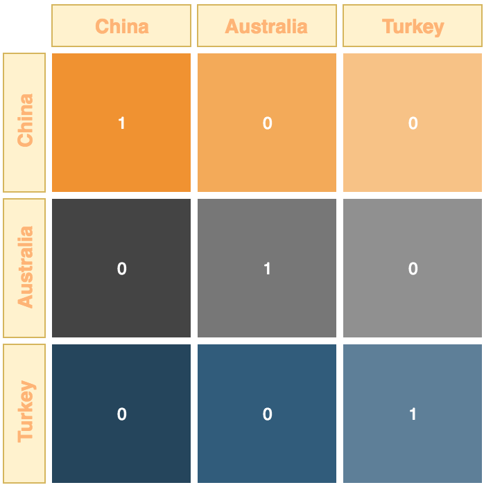
One-hot Encoding

This is where we consider a number of recurring categories, perhaps countries for example:

• China
• Australia
• Turkey

Each category (variable) is converted into a dummy variable which is a binary representation for that category. For example:

But why might we do this? One of the main reasons is that many algorithms and scatter-plots just don’t like non-numerical data.

Missing Data

The final piece to the jigsaw is how to deal with small amounts of missing data, for example, perhaps you want to analyse weather data and specifically things like wind speed, rain fall, and hours of sun, yet as you begin to collect this data, you find that the monitoring stating suffered some loss of data at several points throughout the year, the data that is missing is minor, but it is missing all the same. The best way to deal with this is to ‘guess’ the missing data, having some number (based on the numbers around it) is better than simply discarding the row, furthermore, if you had a small data-set, then every row is precious.

Depending on the types of data you need to ‘guess’ might dictate how you go about this, but here are some possibilities.

Mode Value

You can approximate the missing data using the mode average. The mode is the single most common variable value in this set of data. This works best with categorical data (positive/negative, true/false, simple rating systems etc).

Median Value

Another option is to use the median value. This is essentially the data from the middle of the data-set. This is useful for continuous variables, variables that can move a lot and have an infinite number of contributory variables, such as house prices, or perhaps, stock prices.

The Weather example…

Just to come back to the Weather example, neither the mode or the median over the entire data-set would be suitable for missing data, unless your data range is relatively well confined (a single month, or perhaps a single season), should you consider an entire year or a more, then the missing data would have to be dealt with in monthly or seasonal segments as this will represent a truer reflection of the likely weather during this period of time.

Tags

• Machine Learning
• Data Science
• Data Scrubbing
• One Hot Encoding